使用蒙特卡洛方案为奇异期权定价的观察
一、奇异期权
奇异期权(Exotic Options)是场外交易 (OTC),这意味着它们是由相关交易对手设计的,不能作为交易所交易合约使用。奇异期权包括具有比普通期权更复杂的定价和对冲功能的合约。通常会将市场价格的“隐含”波动性纳入到奇异期权的定价模型中。
奇异期权可以通过以下性质来区别:
1、时间依赖性
比如,离散现金流必然涉及时间依赖性。另一个例子,可能只允许在特定日期或特定时间段提前行权。百慕大期权就具胡这种间歇性的提前行权的特点。
时间依赖具有以下特点:
- 这些期权合约具有时间不一样性;
- 在特定时间点的期权价值或greeks存在跳跃性;
- 在数值方案中的时间离散化问题。
2、现金流
标的资产可能存在现金流,比如:合约可以是债券,付款可以是票息。
不同合约的现金流可能是离散的,也可能是连续的。用以下表达式:
![]()
3、路径依赖
路径依赖合约的收益和价值取决于资产价格路径的历史。
路径依赖主要有两种形式:强路径依赖(如:亚式期权)、弱路径依赖(如:障碍期权)。
4、维度
维数是指基础自变量的数量。
二维:
香草期权有两个独立变量 S 和 t。弱路径依赖合约与其非路径依赖合约具有相同数量的维度,即障碍看涨期权与普通看涨期权具有相同的两个维度。
多维度:
强路径依赖和更多随机源时都会引入更多的变量。
5、阶数
香草期权是一阶的。 它的收益仅取决于基础资产。更高阶期权的收益和价值取决于另一个期权的价值的期权。
亚式期权是奇异期权的一种。其收益取决于标的资产在到期前一段时间内的平均价值。它们具有很强的路径依赖性。它们在到期前的价值取决于所采取的路径。
二、 期权的定价
期权的定价方法有两种:
1、通过模拟定价,蒙特卡罗方法;
蒙特卡罗方法是一种非常通用且强大的技术。
它适合下面几种情况:
- 当有大量维度时,很好用;
- 对于偏微分方程方法难以建立的依赖路径的合约(即使是低维的),很有用;
- 某些模型(例如 HJM)是为蒙特卡罗构建的,不容易(或不可能)编写为 PDE。
蒙特卡罗方法主要缺点是很难使用蒙特卡罗模拟对带有嵌入式决策的选项进行估值。
2、偏微分方程和有限差分法:
偏微分方程方法将期权的估值转化为偏微分方程的解。是合同定价的最佳方法之一。
三、亚式期权
亚式期权是奇异期权的一种。其收益取决于标的资产在到期前一段时间内的平均价值。它们具有很强的路径依赖性。它们在到期前的价值取决于所采取的路径。用于计算期权收益的平均值可以用多种不同的方式定义。例如,它可以是算术平均或几何平均。对期权数据可以使用连续采样,以便使用给定时期内的每个已实现资产价格。 更常见的是,出于实际和法律原因,数据通常是离散的采样。
四、亚式期权的定价
今天我们尝试使用蒙特卡罗模拟的方法对亚式期权进行定价,并分析与观察。通过在风险中性随机游走下获取预期收益的现值来评估 Black–Scholes 中的期权。表达式如下:
dS = rS dt + σS dX
这只是通常的对数正态随机游走,使用的是无风险利率而不是实际利率。
期权的公允价值可以这样计算:对于许多的路径,计算每条路径的收益——这意味着计算路径依赖量的值,然后取所有路径的平均收益,最后取该平均值的现值。
使用蒙特卡洛方法进行期权定价的步骤:
第 1 步:在风险中性世界中模拟标的资产可能的N条价格路径;
第 2 步:计算每个价格路径的期权收益;
第 3 步:计算所有路径的平均收益,并以此平均收益确定期权价格。
五、使用python实现亚式期权的定价
1、首先载入必要的包
%matplotlib notebook

# Importing libraries
import pandas as pd
from numpy import *
import time
from tabulate import tabulate

# Libraries for plotting
import matplotlib.pyplot as plt
%matplotlib inline

import cufflinks as cf
cf.set_config_file(offline=True)
2、初始化示例
亚式期权定价的过程中,需要一些参数,这里我们先进行对这些参数进行赋值。
# Result set
ResultList = [] # Asian Option
ResultListLO = [] # Lookback Option

# Set the label list when printing
# Asian Option
Header = ['S0', 'rate', 'sigma', 'T-t', 'n_sims', 'mc', 'CallValue', 'PutValue', 'RunTime']
# Lookback Option
HeaderLO = ['S0', 'rate', 'sigma', 'T-t', 'n_sims', 'kinds', 'CallValue', 'PutValue']

# Todayís stock price S0
S0 = 100
# Strike E
Se = 100
# Time to expiry (T - t)
horizon = 1
# volatility
sigma = 0.2
# constant risk-free interest rate r
r = 0.05
3、功能函数
蒙特卡罗模拟对亚式期权进行定价,通过在风险中性随机游走下获取预期收益的现值。我们定义一个函数实现随机游走的功能。
def simulate_path(s0, mu, sigma, horizon, timesteps=252, n_sims=100000, mc_type=None, vr_type=None):

    # mc_type: Monte Carlo simulation method
    # vr_type: Variance reduction techniques
    #        None: Do not use;
    #        'AV': antithetic variates.

    # Set the random seed for reproducibility
    # Same seed leads to the same set of random values
    random.seed(10000)

    # Read parameters
    S0 = s0         # initial spot level
    r = mu          # mu = rf in risk neutral framework
    T = horizon     # time horizion
    t = timesteps   # number of time steps
    n = n_sims      # number of simulation

    # Define dt
    dt = T/t        # length of time interval

    # Simulating 'n' asset price paths with 't' timesteps
    S = zeros((t+1, n))
    S[0] = S0

    # antithetic variates
    if vr_type == "AV":
        Y = zeros((t+1, n))
        Y[0] = S0
    else:
        Y = arange(1)

    for i in range(1, t+1):
        z = random.standard_normal(n)     # psuedo random numbers
        if mc_type == "EM":
            # Use the Euler-Maruyama
            S[i] = S[i-1] * (1 + r * dt + sigma * sqrt(dt) * z)

            if vr_type == "AV":
                # antithetic variates
                Y[i] = Y[i-1] * (1 + r * dt + sigma * sqrt(dt) * -z)

        else:
            S[i] = S[i-1] * exp((r - 0.5 * sigma ** 2) * dt + sigma * sqrt(dt) * z) # vectorized operation per timesteps

            if vr_type == "AV":
                # antithetic variates
                Y[i] = Y[i-1] * exp((r - 0.5 * sigma ** 2) * dt + sigma * sqrt(dt) * -z)

    return pd.DataFrame(S), pd.DataFrame(Y)
我们还需要定义一个根据亚式期权性质生成蒙特卡罗模拟的路径的函数。
def asin_option(S0, r, sigma, horizon, timesteps=252, n_sims=100000, mc_type=None, vr_type=None):

    # mc_type: Monte Carlo simulation method
    # vr_type: Variance reduction techniques
    #        None: Do not use;
    #        'AV': antithetic variates.

    # start the timer
    time_start = time.time()

    # MC
    spath, ypath = simulate_path(S0, r, sigma, horizon, timesteps=timesteps, n_sims=n_sims,
                                 mc_type=mc_type, vr_type=vr_type)

    # Average price
    A1 = spath.mean(axis=0)

    # Calculate the discounted value of the expeced payoff
    C1 = exp(-r*horizon) * mean(maximum(A1 - Se, 0))
    P1 = exp(-r*horizon) * mean(maximum(Se - A1, 0))

    if vr_type == "AV":
        # Average price
        A2 = ypath.mean(axis=0)

        # Calculate the discounted value of the expeced payoff
        C2 = exp(-r*horizon) * mean(maximum(A2 - Se, 0))
        C0 = (C1+C2)/2

        P2 = exp(-r*horizon) * mean(maximum(Se - A2, 0))
        P0 = (P1+P2)/2
    else:
        C0 = C1
        P0 = P1

    # Calculate running time
    time_run = time.time() - time_start

    # Add calculation results to the list
    ResultList.append([S0, r, sigma, horizon, n_sims, mc_type, C0, P0, time_run])

    return spath, ypath
4、初步对不同的参数进行定价并进行观察
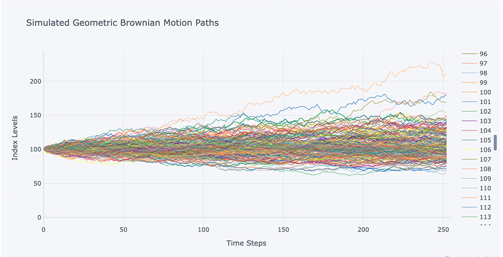
# Default method and no variance reduction scheme
spath, ypath = asin_option(S0, r, sigma, horizon, mc_type=None, n_sims=100000, vr_type=None)

# Show the simulation path with graphs

spath.iloc[:,:200].iplot(xTitle='Time Steps',
                         yTitle='Index Levels',
                         title='Simulated Geometric Brownian Motion Paths')
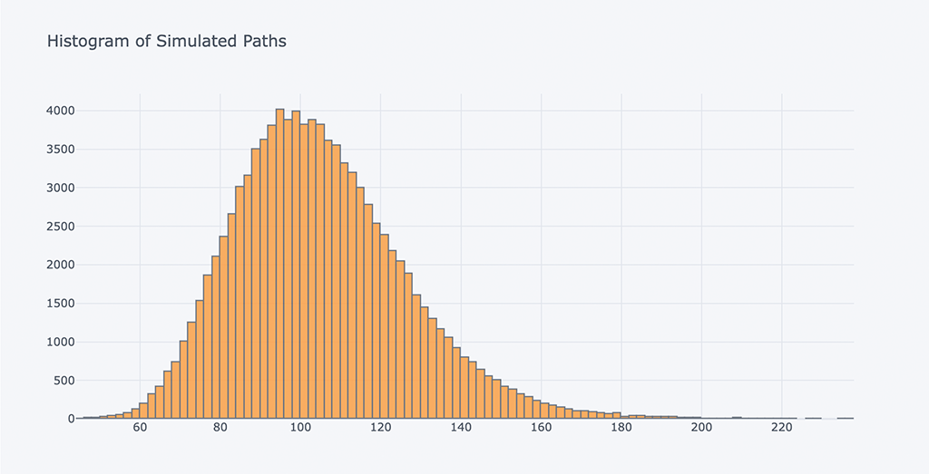
# Histogram of Simulated Paths
# Plot the histogram of the simulated price path at maturity
spath.iloc[-1].iplot(kind='histogram',
                     bins=100,
                     title= 'Histogram of Simulated Paths')
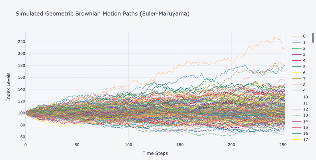
# Euler-Maruyama and no variance reduction scheme

spath, ypath = asin_option(S0, r, sigma, horizon, mc_type='EM', n_sims=100000, vr_type=None)

# Show the simulation path with graphs
spath.iloc[:,:200].iplot(xTitle='Time Steps',
                         yTitle='Index Levels',
                         title='Simulated Geometric Brownian Motion Paths (Euler-Maruyama)')
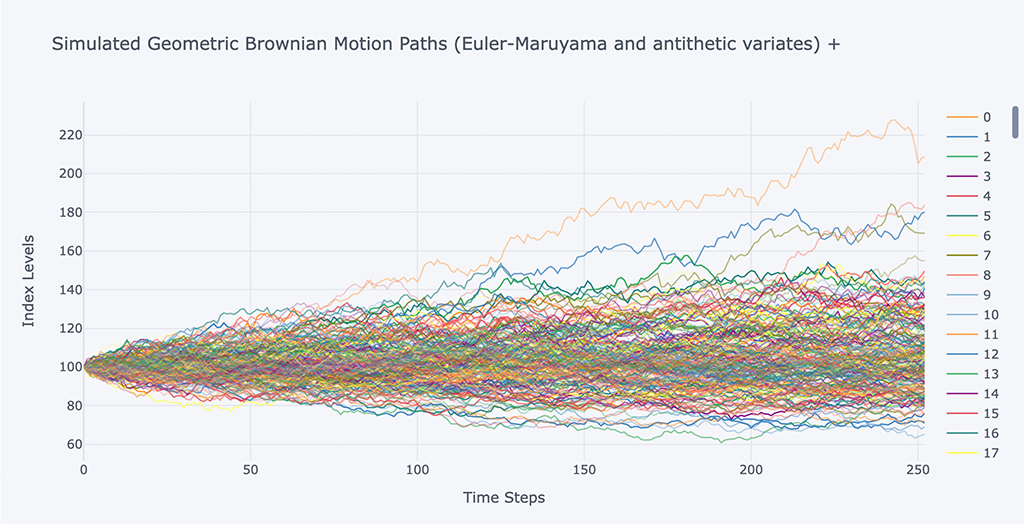
# Euler-Maruyama and use antithetic variates to reduce variance
spath, ypath = asin_option(S0, r, sigma, horizon, mc_type='EM', n_sims=100000, vr_type='AV')
# Graphically show the simulation path in the positive direction
spath.iloc[:,:200].iplot(xTitle='Time Steps',
yTitle='Index Levels',
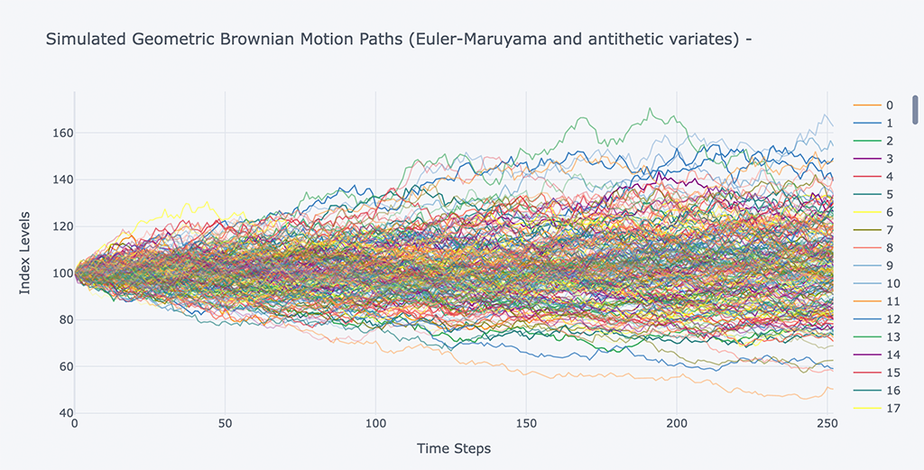
title='Simulated Geometric Brownian Motion Paths (Euler-Maruyama and antithetic variates) +')
# Graphically show the reverse simulation path
ypath.iloc[:,:200].iplot(xTitle='Time Steps',
                         yTitle='Index Levels',
                         title='Simulated Geometric Brownian Motion Paths (Euler-Maruyama and antithetic variates) -')
我们现在对比以上三种场景的结果。
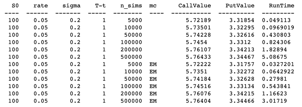
# The last one is to use antithetic variates to reduce variance.
print(tabulate(ResultList,Header))
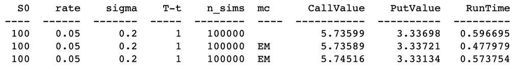
可以看出,在同样进行100K 次模拟的情况下,得出的Call Value和Put Value相差不大,在运行时间略有差别,再继续观察更多的场景。
5、深入观察更多不同参数的变化对定价结果及执行速度的影响
5.1观察不使用减少方差方案时,模拟次数的不同对定价结果的影响
ResultList = []
spath, ypath = asin_option(S0, r, sigma, horizon, mc_type=None, n_sims=10000, vr_type=None)
spath, ypath = asin_option(S0, r, sigma, horizon, mc_type=None, n_sims=50000, vr_type=None)
spath, ypath = asin_option(S0, r, sigma, horizon, mc_type=None, n_sims=100000, vr_type=None)
spath, ypath = asin_option(S0, r, sigma, horizon, mc_type=None, n_sims=200000, vr_type=None)
spath, ypath = asin_option(S0, r, sigma, horizon, mc_type=None, n_sims=500000, vr_type=None)
spath, ypath = asin_option(S0, r, sigma, horizon, mc_type=None, n_sims=1000000, vr_type=None)
spath, ypath = asin_option(S0, r, sigma, horizon, mc_type='EM', n_sims=10000, vr_type=None)
spath, ypath = asin_option(S0, r, sigma, horizon, mc_type='EM', n_sims=50000, vr_type=None)
spath, ypath = asin_option(S0, r, sigma, horizon, mc_type='EM', n_sims=100000, vr_type=None)
spath, ypath = asin_option(S0, r, sigma, horizon, mc_type='EM', n_sims=200000, vr_type=None)
spath, ypath = asin_option(S0, r, sigma, horizon, mc_type='EM', n_sims=500000, vr_type=None)
spath, ypath = asin_option(S0, r, sigma, horizon, mc_type='EM', n_sims=1000000, vr_type=None)
# Print the values
print(tabulate(ResultList,Header))
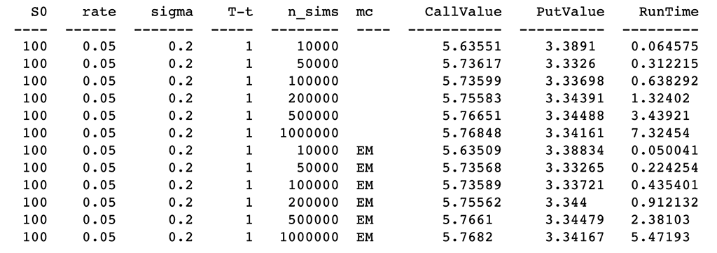
基于以上结果,亚洲期权的两种蒙特卡洛模拟方法进行如下分析:
a. 从精度对比分析来看,看涨期权价值(Call Value)和看跌期权价值(Put Value)的结果,两者相差很小,结果高度相似。
b. 模拟次数越大,看涨期权价值(Call Value)和看跌期权价值(Put Value)越趋向平滑。
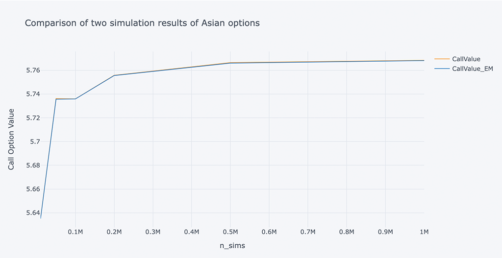
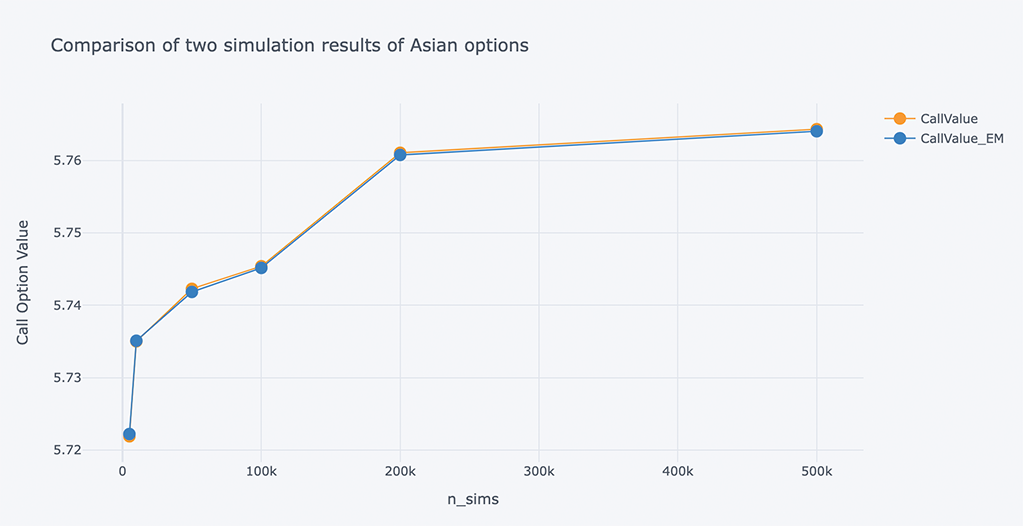
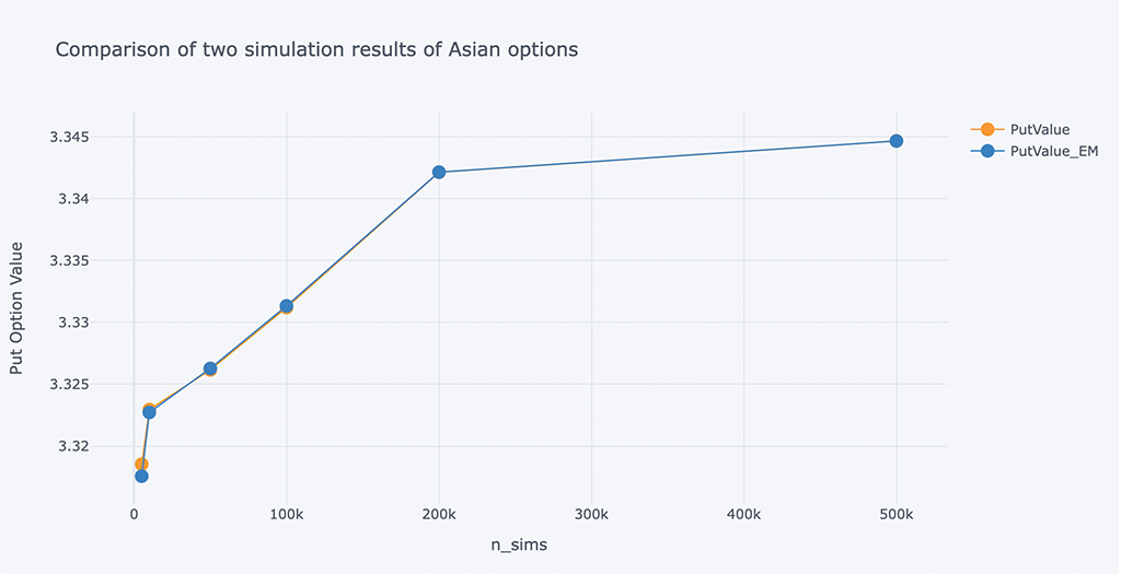
把结果的对比用图表的方式打印出来,我们可以看到更加直观的表现。
# A chart comparing the Call Option Value of two simulations of Asian options

outdata = pd.DataFrame(ResultList, columns=Header)
outdata2 = column_stack((outdata[0:6][['n_sims', 'CallValue']].values,
                         outdata[6:12][['CallValue']].values))
outdata2 = pd.DataFrame(outdata2, columns=['n_sims', 'CallValue', 'CallValue_EM'])

outdata2.iplot(x='n_sims',
               y=['CallValue','CallValue_EM'],
               xTitle='n_sims',
               yTitle='Call Option Value',
               title='Comparison of two simulation results of Asian options')
# A chart comparing the Put Option Value of two simulations of Asian options

outdata = pd.DataFrame(ResultList, columns=Header)
outdata2 = column_stack((outdata[0:6][['n_sims', 'PutValue']].values,
                         outdata[6:12][['PutValue']].values))
outdata2 = pd.DataFrame(outdata2, columns=['n_sims', 'PutValue', 'PutValue_EM'])

outdata2.iplot(x='n_sims',
               y=['PutValue','PutValue_EM'],
               xTitle='n_sims',
               yTitle='Put Option Value',
               title='Comparison of two simulation results of Asian options')
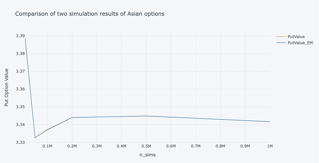
结合上图,更直观的表现了我们上面的两个观点,模拟次数越多越能获得更好的期权价值。
结合上面这组数据,当 10k 到 20K 模拟时估计值有很大提高,使用 500K 模拟时估计改进趋于稳定。同时我们也要考虑模拟的时间,在时间与精度之间找到一个平衡点。
5.2 观察使用减少方差方案时,模拟次数的不同对定价结果的影响
ResultList1 = ResultList.copy()
ResultList = []
spath, ypath = asin_option(S0, r, sigma, horizon, mc_type=None, n_sims=5000, vr_type='AV')
spath, ypath = asin_option(S0, r, sigma, horizon, mc_type=None, n_sims=10000, vr_type='AV')
spath, ypath = asin_option(S0, r, sigma, horizon, mc_type=None, n_sims=50000, vr_type='AV')
spath, ypath = asin_option(S0, r, sigma, horizon, mc_type=None, n_sims=100000, vr_type='AV')
spath, ypath = asin_option(S0, r, sigma, horizon, mc_type=None, n_sims=200000, vr_type='AV')
spath, ypath = asin_option(S0, r, sigma, horizon, mc_type=None, n_sims=500000, vr_type='AV')
spath, ypath = asin_option(S0, r, sigma, horizon, mc_type='EM', n_sims=5000, vr_type='AV')
spath, ypath = asin_option(S0, r, sigma, horizon, mc_type='EM', n_sims=10000, vr_type='AV')
spath, ypath = asin_option(S0, r, sigma, horizon, mc_type='EM', n_sims=50000, vr_type='AV')
spath, ypath = asin_option(S0, r, sigma, horizon, mc_type='EM', n_sims=100000, vr_type='AV')
spath, ypath = asin_option(S0, r, sigma, horizon, mc_type='EM', n_sims=200000, vr_type='AV')
spath, ypath = asin_option(S0, r, sigma, horizon, mc_type='EM', n_sims=500000, vr_type='AV')
# Print the values
print(tabulate(ResultList,Header))
# A chart comparing the Call Option Value of two simulations of Asian options

outdata = pd.DataFrame(ResultList, columns=Header)
outdata2 = column_stack((outdata[0:6][['n_sims', 'CallValue']].values,
                         outdata[6:12][['CallValue']].values))
outdata2 = pd.DataFrame(outdata2, columns=['n_sims', 'CallValue', 'CallValue_EM'])

outdata2.iplot(x='n_sims',
               y=['CallValue','CallValue_EM'],
               mode='lines+markers',
               xTitle='n_sims',
               yTitle='Call Option Value',
               title='Comparison of two simulation results of Asian options')
# A chart comparing the Put Option Value of two simulations of Asian options

outdata = pd.DataFrame(ResultList, columns=Header)
outdata2 = column_stack((outdata[0:6][['n_sims', 'PutValue']].values,
                         outdata[6:12][['PutValue']].values))
outdata2 = pd.DataFrame(outdata2, columns=['n_sims', 'PutValue', 'PutValue_EM'])

outdata2.iplot(x='n_sims', y=['PutValue','PutValue_EM'],
               mode='lines+markers',
               xTitle='n_sims', yTitle='Put Option Value',
               title='Comparison of two simulation results of Asian options')
在仅模拟5K次时,对比发现加入减少方差的方案,可以比较好的提高定价精度。可以使用更少的模拟次数而达到更好的定价精度。
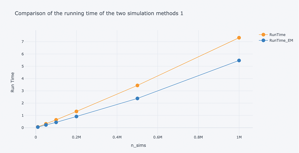
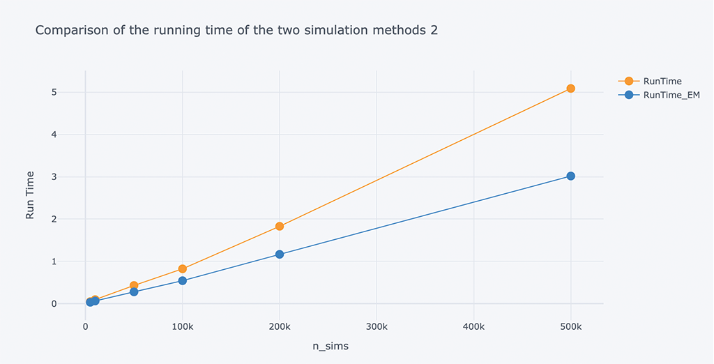
5.3 对比以上不同方案运行的时间
在使用蒙特卡罗模拟方法进行期权定价时,定价所需的时间也很关键。应该在可接受的精度范围内,尽可能减少定价所需时间。
# A chart Comparison of the running time of the two simulation methods

outdata = pd.DataFrame(ResultList1, columns=Header)
outdata2 = column_stack((outdata[0:6][['n_sims', 'RunTime']].values,
                         outdata[6:12][['RunTime']].values))
outdata2 = pd.DataFrame(outdata2, columns=['n_sims', 'RunTime', 'RunTime_EM'])

outdata2.iplot(x='n_sims', y=['RunTime', 'RunTime_EM'],
               mode='lines+markers',
               xTitle='n_sims', yTitle='Run Time',
               title='Comparison of the running time of the two simulation methods 1')
# A chart Comparison of the running time of the two simulation methods

outdata = pd.DataFrame(ResultList, columns=Header)
outdata2 = column_stack((outdata[0:6][['n_sims', 'RunTime']].values,
                         outdata[6:12][['RunTime']].values))
outdata2 = pd.DataFrame(outdata2, columns=['n_sims', 'RunTime', 'RunTime_EM'])

outdata2.iplot(x='n_sims', y=['RunTime', 'RunTime_EM'],
               mode='lines+markers',
               xTitle='n_sims',
               yTitle='Run Time',
               title='Comparison of the running time of the two simulation methods 2')
# Comparison chart of running time and accuracy of the four schemes
outdata = pd.DataFrame(ResultList, columns=Header)
outdata1 = pd.DataFrame(ResultList1, columns=Header)

plt.figure(num=3,figsize=(15,10))
plt.plot(outdata[0:6][['RunTime']], outdata[0:6][['CallValue']],
         color='red', linewidth=1, label="Default")
plt.plot(outdata[6:12][['RunTime']], outdata[6:12][['CallValue']],
         color='gold', linewidth=1, label="EM")
plt.plot(outdata1[0:6][['RunTime']], outdata1[0:6][['CallValue']],
         color='green', linewidth=1, label="default  AV")
plt.plot(outdata1[6:12][['RunTime']], outdata1[6:12][['CallValue']],
         color='blue', linewidth=1, label="EM  AV")
plt.xlabel('Run Time')
plt.ylabel('Call Option Value')
plt.title('Time and OptionValue')
plt.show()
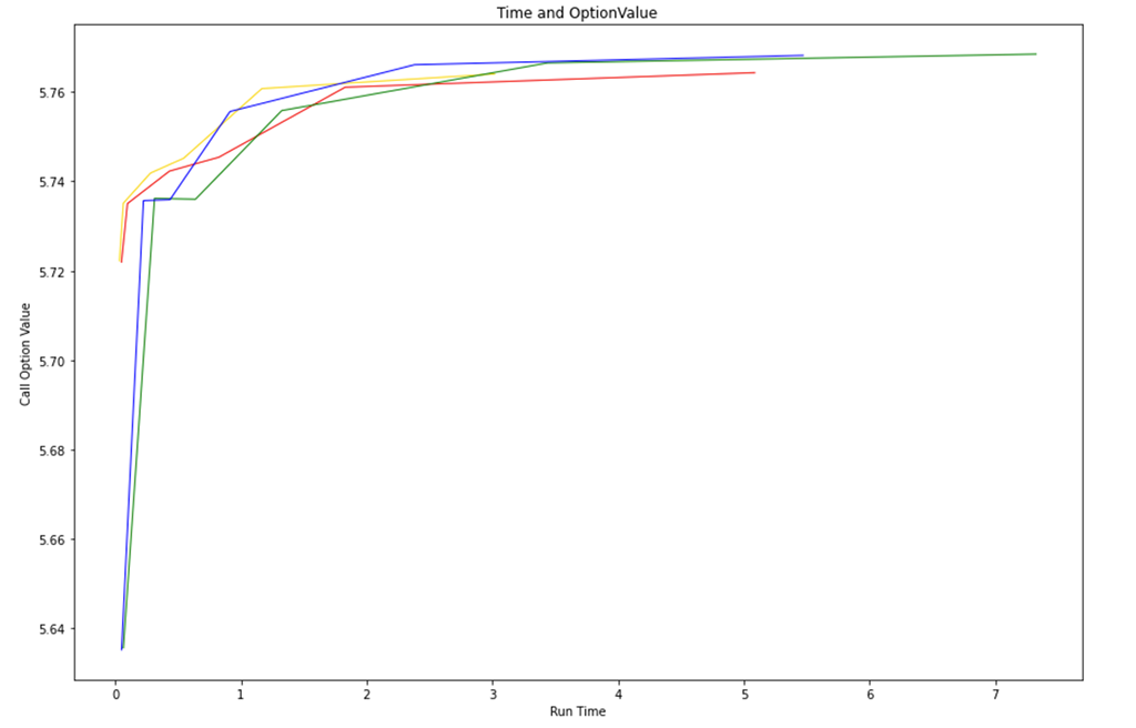
根据上图中的蓝线可以看出,Euler-Maruyama方案在相同精度下计算时间更短,效率更高。
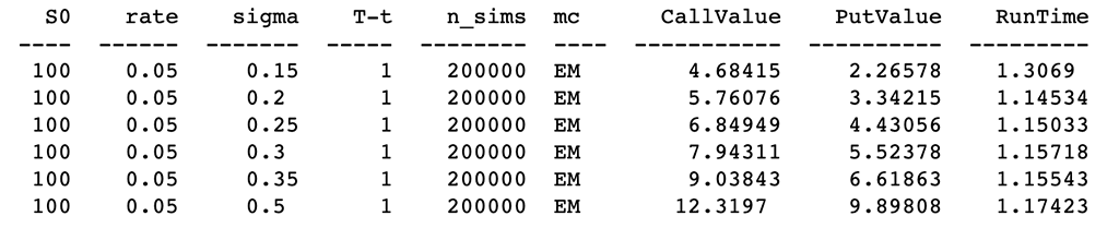
5.4 不同波动率的影响
分析不同波动率的影响,假设有 6 种不同的波动率,比较模拟路径和结果。
ResultList = []
spath, ypath = asin_option(S0, r, 0.15, horizon, mc_type='EM', n_sims=200000, vr_type='AV')
spath, ypath = asin_option(S0, r, 0.2, horizon, mc_type='EM', n_sims=200000, vr_type='AV')
spath, ypath = asin_option(S0, r, 0.25, horizon, mc_type='EM', n_sims=200000, vr_type='AV')
spath, ypath = asin_option(S0, r, 0.3, horizon, mc_type='EM', n_sims=200000, vr_type='AV')
spath, ypath = asin_option(S0, r, 0.35, horizon, mc_type='EM', n_sims=200000, vr_type='AV')
spath, ypath = asin_option(S0, r, 0.5, horizon, mc_type='EM', n_sims=200000, vr_type='AV')
# Print the values
print(tabulate(ResultList,Header))
# Chart of changes in volatility and option value
outdata = pd.DataFrame(ResultList, columns=Header)
outdata[['sigma', 'CallValue','PutValue']].iplot(x='sigma', y=['CallValue', 'PutValue'],
                                                             mode='lines+markers',
                                                             title='Volatility and changes in option value',
                                                             xTitle='sigma', yTitle='Option Value')
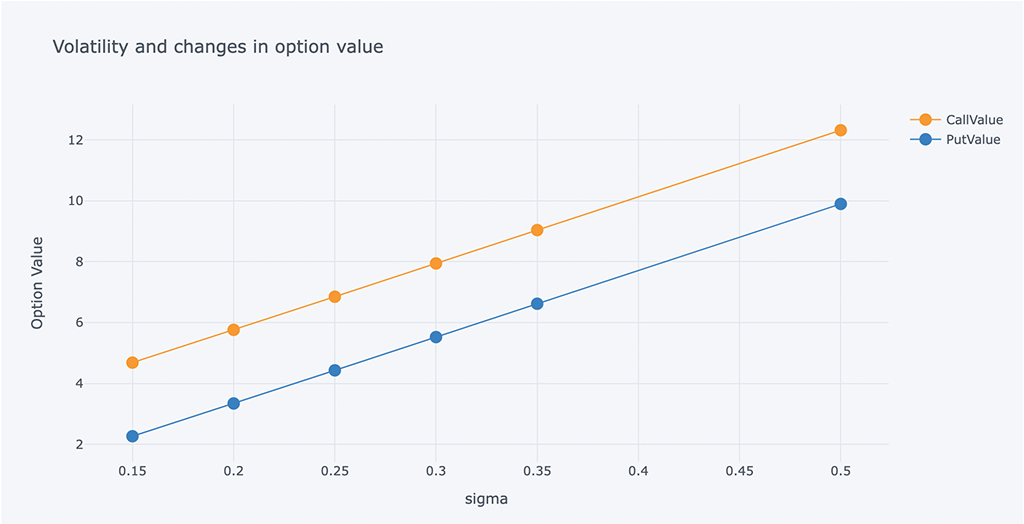
可以看出在其他参数不变的情况下,从不同的波动率可以看出,期权价值随着波动率的增大而增加,随着波动率的减小而减小。
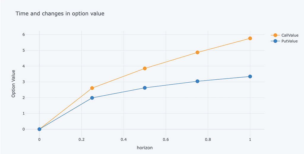
5.5 时间变化的影响
下面以季度为间隔分析时间的影响。
# Calculated according to the time of each quarter
ResultList = []
for i in arange(1, -0.001, -0.25):
    spath, ypath = asin_option(S0, r, sigma, i, mc_type='EM', n_sims=200000, vr_type='AV')
# Print the values
print(tabulate(ResultList,Header))
# Chart of changes in volatility and option value
outdata = pd.DataFrame(ResultList, columns=Header)
outdata[['T-t', 'CallValue','PutValue']].iplot(x='T-t',
                                               y=['CallValue', 'PutValue'],
                                               mode='lines+markers',
                                               xTitle='horizon',
                                               yTitle='Option Value',
                                               title='Time and changes in option value')
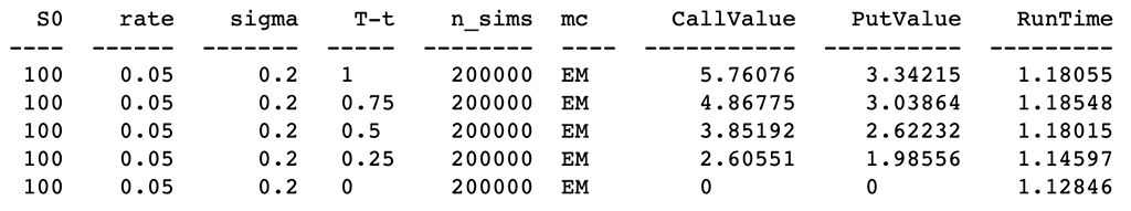
5.6 无风险利率对期权价值的影响
从负利率到正利率,分析无风险利率对期权价值的影响。
# Different risk-free interest rates to calculate option value
ResultList = []
for i in arange(-0.02, 0.06, 0.01):
    spath, ypath = asin_option(S0, i, sigma, horizon, mc_type='EM', n_sims=200000, vr_type='AV')
# Print the values
print(tabulate(ResultList,Header))
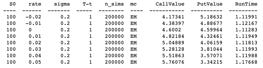
# Chart of Risk-free interest rate and option value
outdata = pd.DataFrame(ResultList, columns=Header)
outdata[['rate', 'CallValue','PutValue']].iplot(x='rate',
                                                y=['CallValue', 'PutValue'],
                                                mode='lines+markers',
                                                xTitle='rate', yTitle='Option Value',
                                                title='Risk-free interest rate and option value')
在其他参数不变的前提下,当无风险利率上升时,PUT 期权价值下降。 当无风险利率增加时,看涨期权价值增加。看跌期权和看涨期权在零处交叉。
5.7 观察不同的初始标的资产价格
分析初始标的资产价格对期权价值的影响。
# Different risk-free interest rates to calculate option value
ResultList = []
for i in arange(0, 200, 10):
    spath, ypath = asin_option(i, r, sigma, horizon, mc_type='EM', n_sims=200000, vr_type='AV')
# Print the values
print(tabulate(ResultList,Header))
# Chart of Risk-free interest rate and option value
outdata = pd.DataFrame(ResultList, columns=Header)
outdata[['S0', 'CallValue','PutValue']].iplot(x='S0', y=['CallValue', 'PutValue'],
                                              mode='lines+markers',
                                              xTitle='S0', yTitle='Option Value',
                                              title='S0 and option value')
def lookback_option(S0, r, sigma, horizon, timesteps=252, n_sims=100000, mc_type=None, vr_type=None, lo_type='FLOATING'):

    # mc_type: Monte Carlo simulation method
    # vr_type: Variance reduction techniques
    #        None: Do not use;
    #        'AV': antithetic variates.
    # lo_type: Lookback Option type
    #        'FLOATING': with floating strike.
    #        ‘FIXED’: with fixed strike.

    # start the timer
    time_start = time.time()

    # MC
    spath, ypath = simulate_path(S0, r, sigma, horizon, timesteps=timesteps, n_sims=n_sims,
                                 mc_type=mc_type, vr_type=vr_type)

    # max price and min price
    max_s = spath.max(axis=0)
    min_s = spath.min(axis=0)

    # Calculate the discounted value of the expeced payoff
    if lo_type == "FIXED":
        # With fixed strike
        C1 = exp(-r*horizon) * mean(maximum(max_s - Se, 0))
        P1 = exp(-r*horizon) * mean(maximum(Se - min_s, 0))

    else:
        # With floating strike
        C1 = exp(-r*horizon) * mean(maximum(spath.iloc[-1] - min_s, 0))
        P1 = exp(-r*horizon) * mean(maximum(max_s - spath.iloc[-1], 0))

    if vr_type == "AV":
        # Average price
        max_y = spath.max(axis=0)
        min_y = spath.min(axis=0)

        # Calculate the discounted value of the expeced payoff
        if lo_type == "FIXED":
            # With fixed strike
            C2 = exp(-r*horizon) * mean(maximum(max_y - Se, 0))
            P2 = exp(-r*horizon) * mean(maximum(Se - min_y, 0))

        else:
            # With floating strike
            C2 = exp(-r*horizon) * mean(maximum(ypath.iloc[-1] - min_y, 0))
            P2 = exp(-r*horizon) * mean(maximum(max_y - ypath.iloc[-1], 0))

        C0 = (C1+C2)/2
        P0 = (P1+P2)/2
    else:
        C0 = C1
        P0 = P1

    # Calculate running time
    time_run = time.time() - time_start

    # Add calculation results to the list
    ResultListLO.append([S0, r, sigma, horizon, n_sims, lo_type, C0, P0])

    return spath, ypath
# Calculate the discounted value of the expeced payoff
spath, ypath = lookback_option(S0, r, sigma, horizon, mc_type='EM', n_sims=200000, vr_type='AV', lo_type='FLOATING')

# Print the values (FLOATING)
print(tabulate(ResultListLO, HeaderLO))
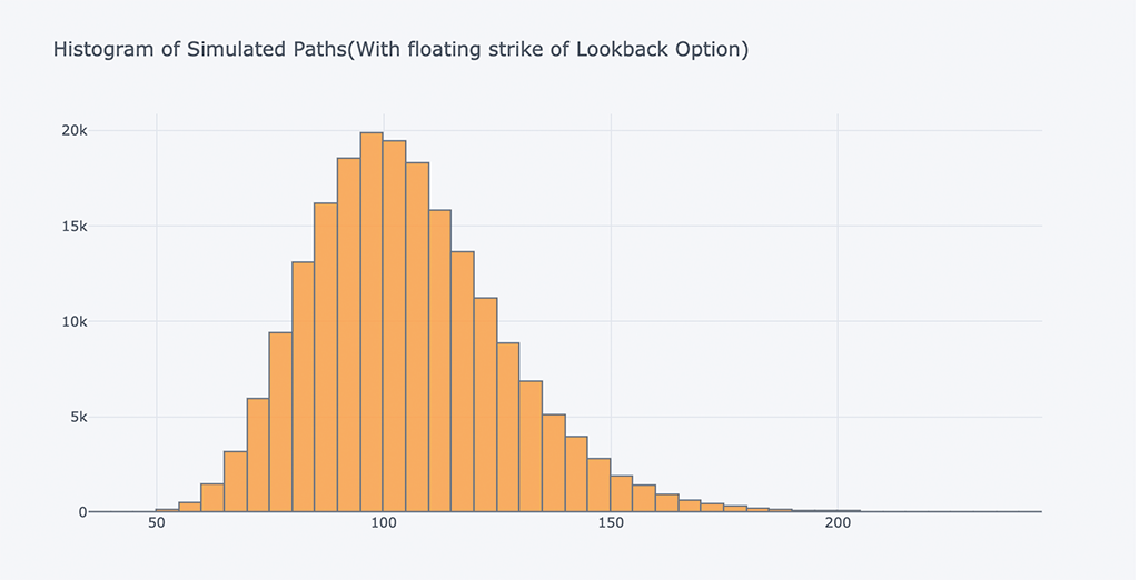
# Plot the histogram of the simulated price path at maturity
spath.iloc[-1].iplot(kind='histogram',
                     bins=100,
                     title= 'Histogram of Simulated Paths(With floating strike of Lookback Option)')
# Plot simulated price paths
spath.iloc[:,:200].iplot(xTitle='Time Steps', yTitle='Index Levels',
                        title='Simulated Geometric Brownian Motion Paths(With floating strike of Lookback Option)')

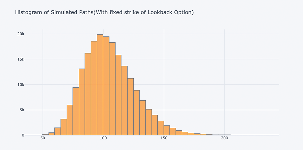
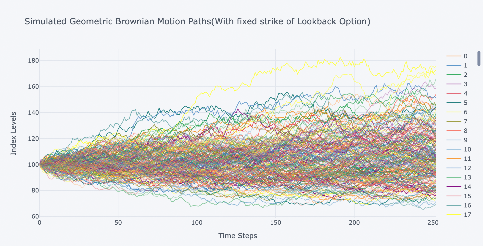
b、固定回望期权:
# Calculate the discounted value of the expeced payoff
spath, ypath = lookback_option(S0, r, sigma, horizon, mc_type='EM', n_sims=200000, vr_type='AV', lo_type='FIXED')

# Print the values(FIXED)
print(tabulate(ResultListLO[-1:], HeaderLO))

# Plot the histogram of the simulated price path at maturity
spath.iloc[-1].iplot(kind='histogram',bins=100,
                     title= 'Histogram of Simulated Paths(With fixed strike of Lookback Option)')
# Plot simulated price paths
spath.iloc[:,:200].iplot(xTitle='Time Steps', yTitle='Index Levels',
                        title='Simulated Geometric Brownian Motion Paths(With fixed strike of Lookback Option)')
对两种回溯期权的定价结果进行比较:
# Print the values
print(tabulate(ResultListLO, HeaderLO))
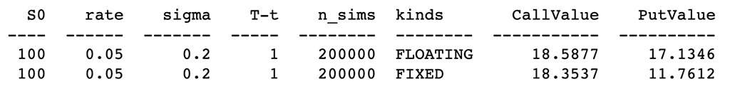
从上面结果可得出:浮动行使价的期权价值将高于固定行使价。
6.2 不同波动率的影响:
假设有 6 种不同的波动率,比较模拟路径和结果。
a、 带有浮动回望期权:
ResultListLO = []
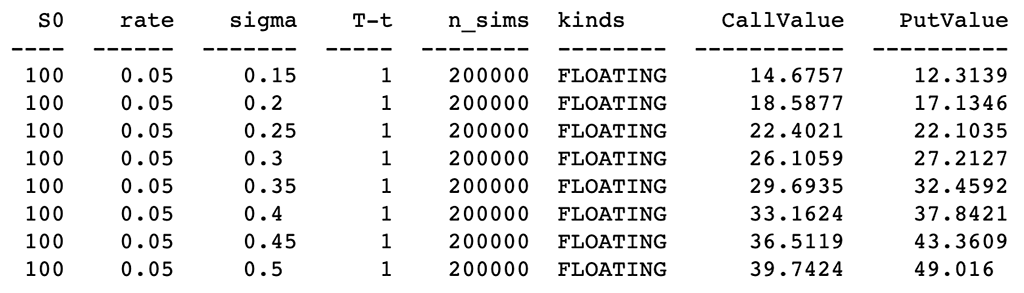
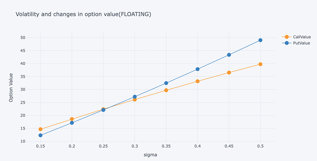
for i in arange(0.15, 0.51, 0.05):
spath, ypath = lookback_option(S0, r, i, horizon, mc_type='EM', n_sims=200000, vr_type='AV', lo_type='FLOATING')
# Print the values
print(tabulate(ResultListLO, HeaderLO))
# Chart of changes in volatility and option value
outdata = pd.DataFrame(ResultListLO, columns=HeaderLO)
outdata[['sigma', 'CallValue','PutValue']].iplot(x='sigma',
                                                 y=['CallValue', 'PutValue'],
                                                 mode='lines+markers',
                                                 xTitle='sigma', yTitle='Option Value',
                                                 title='Volatility and changes in option value(FLOATING)')
b、固定回望期权:
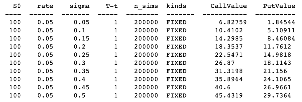
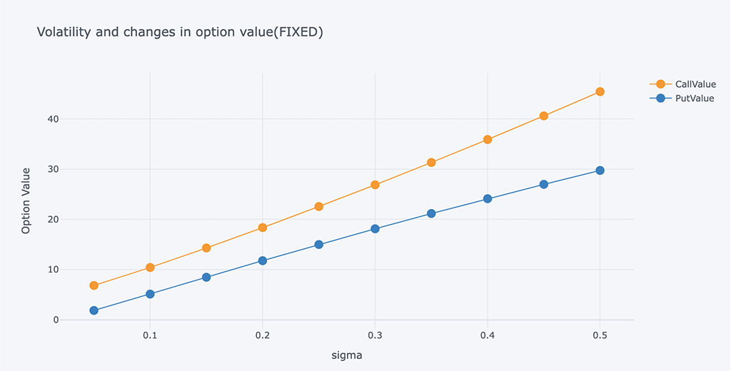
ResultListLO = []
for i in arange(0.05, 0.51, 0.05):
    spath, ypath = lookback_option(S0, r, i, horizon, mc_type='EM', n_sims=200000, vr_type='AV', lo_type='FIXED')
# Print the values
print(tabulate(ResultListLO, HeaderLO))
# Chart of changes in volatility and option value
outdata = pd.DataFrame(ResultListLO, columns=HeaderLO)
outdata[['sigma', 'CallValue','PutValue']].iplot(x='sigma', y=['CallValue', 'PutValue'],
                                                 mode='lines+markers',
                                                 xTitle='sigma', yTitle='Option Value',
                                                 title='Volatility and changes in option value(FIXED)')
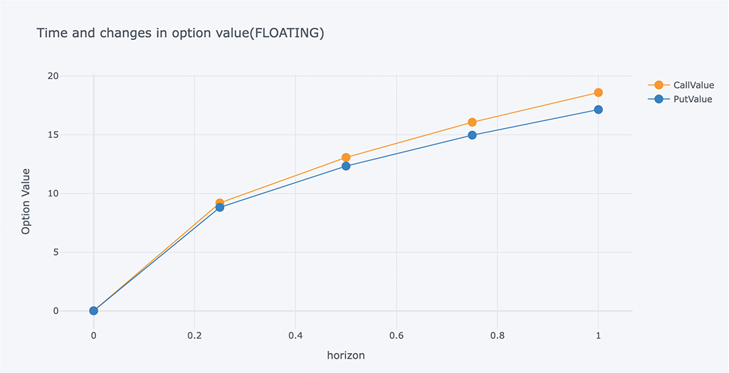
# Calculated according to the time of each quarter
ResultListLO = []
for i in arange(1, -0.001, -0.25):
    spath, ypath = lookback_option(S0, r, sigma, i, mc_type='EM', n_sims=200000, vr_type='AV', lo_type='FLOATING')
# Print the values
print(tabulate(ResultListLO,HeaderLO))
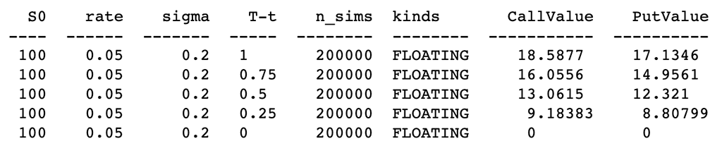
# Chart of changes in volatility and option value
outdata = pd.DataFrame(ResultListLO, columns=HeaderLO)
outdata[['T-t', 'CallValue','PutValue']].iplot(x='T-t',
                                               y=['CallValue', 'PutValue'],
                                               mode='lines+markers',
                                               xTitle='horizon',
                                               yTitle='Option Value',
                                               title='Time and changes in option value(FLOATING)')
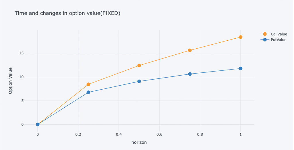
b、固定回望期权:
# Calculated according to the time of each quarter
ResultListLO = []
for i in arange(1, -0.001, -0.25):
    spath, ypath = lookback_option(S0, r, sigma, i, mc_type='EM', n_sims=200000, vr_type='AV', lo_type='FIXED')
# Print the values
print(tabulate(ResultListLO,HeaderLO))
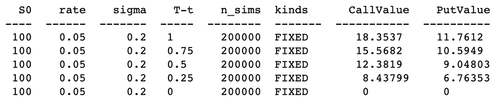
# Chart of changes in volatility and option value
outdata = pd.DataFrame(ResultListLO, columns=HeaderLO)
outdata[['T-t', 'CallValue','PutValue']].iplot(x='T-t',
                                               y=['CallValue', 'PutValue'],
                                               mode='lines+markers',
                                               xTitle='horizon',
                                               yTitle='Option Value',
                                               title='Time and changes in option value(FIXED)')
# Different risk-free interest rates to calculate option value
ResultListLO = []
for i in arange(-0.02, 0.06, 0.01):
    spath, ypath = lookback_option(S0, i, sigma, horizon, mc_type='EM', n_sims=200000, vr_type='AV', lo_type='FLOATING')
# Print the values
print(tabulate(ResultListLO,HeaderLO))
# Chart of Risk-free interest rate and option value
outdata = pd.DataFrame(ResultListLO, columns=HeaderLO)
outdata[['rate', 'CallValue','PutValue']].iplot(x='rate',
y=['CallValue', 'PutValue'],
mode='lines+markers',
xTitle='rate',
yTitle='Option Value',
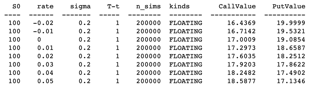
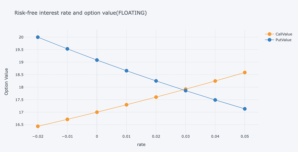
title='Risk-free interest rate and option value(FLOATING)')
b、固定回望期权
# Different risk-free interest rates to calculate option value
ResultListLO = []
for i in arange(-0.02, 0.06, 0.01):
    spath, ypath = lookback_option(S0, i, sigma, horizon, mc_type='EM', n_sims=200000, vr_type='AV', lo_type='FIXED')
# Print the values
print(tabulate(ResultListLO,HeaderLO))
# Chart of Risk-free interest rate and option value
outdata = pd.DataFrame(ResultListLO, columns=HeaderLO)
outdata[['rate', 'CallValue','PutValue']].iplot(x='rate',
y=['CallValue', 'PutValue'],
mode='lines+markers',
xTitle='rate',
yTitle='Option Value',
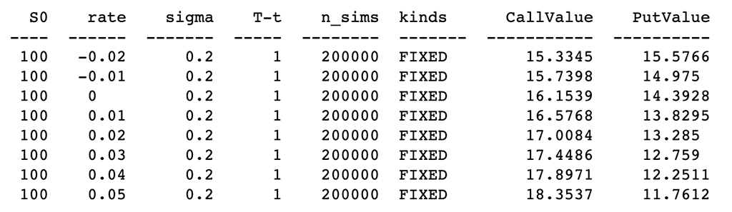
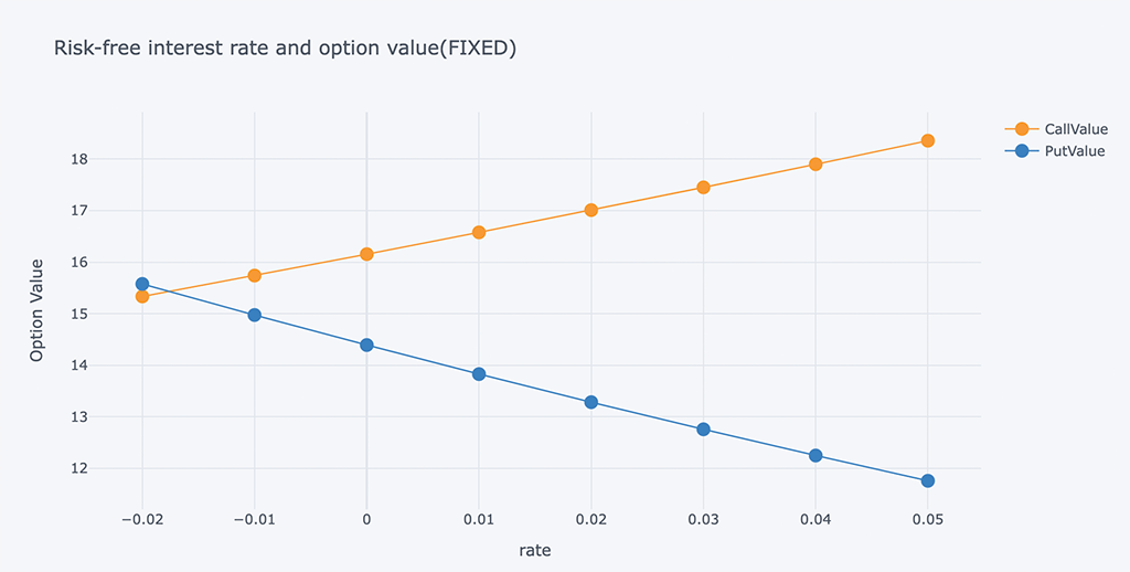
title='Risk-free interest rate and option value(FIXED)')
浮动追溯期权的看跌期权和看涨期权的交叉在0.03左右。
固定追溯期权的看跌期权和看涨期权的交叉点在-0.018左右。
6.5 观察不同的 S0
分析初始标的资产价格对期权价值的影响。
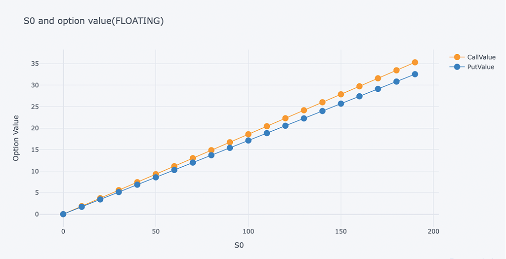
a、带有浮动回望期权:
# Different risk-free interest rates to calculate option value
ResultListLO = []
for i in arange(0, 200, 10):
    spath, ypath = lookback_option(i, r, sigma, horizon, mc_type='EM', n_sims=200000, vr_type='AV', lo_type='FLOATING')
# Print the values
print(tabulate(ResultListLO, HeaderLO))
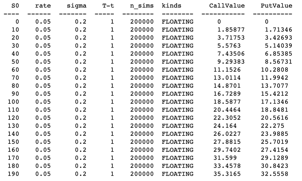
# Chart of Risk-free interest rate and option value
outdata = pd.DataFrame(ResultListLO, columns=HeaderLO)
outdata[['S0', 'CallValue','PutValue']].iplot(x='S0',
                                              y=['CallValue', 'PutValue'],
                                              mode='lines+markers',
                                              xTitle='S0',
                                              yTitle='Option Value',
                                              title='S0 and option value(FLOATING)')
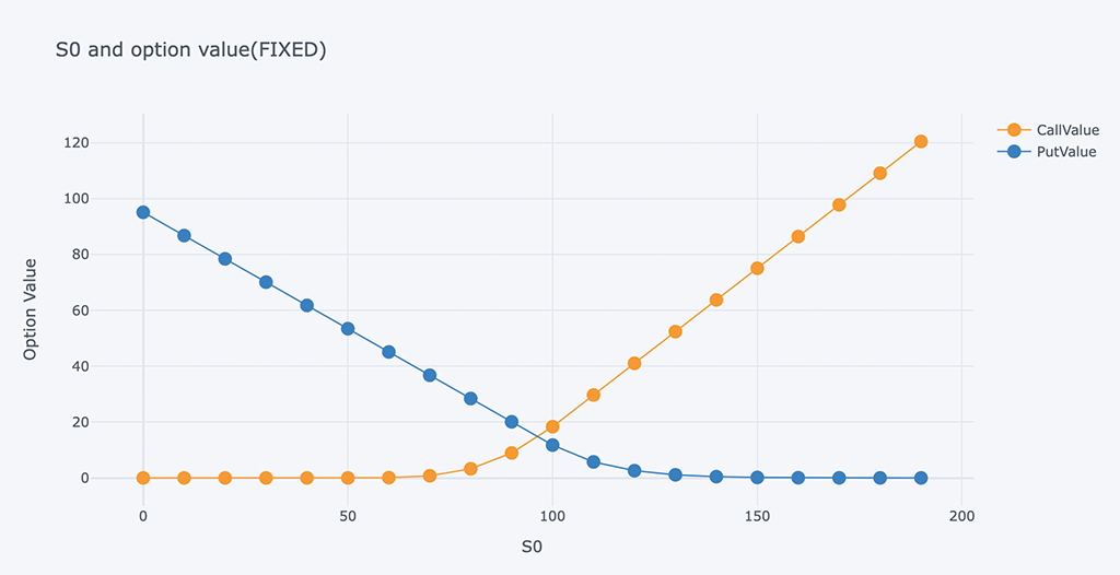
b、 固定回望期权:
# Different risk-free interest rates to calculate option value
ResultListLO = []
for i in arange(0, 200, 10):
    spath, ypath = lookback_option(i, r, sigma, horizon, mc_type='EM', n_sims=200000, vr_type='AV', lo_type='FIXED')
# Print the values
print(tabulate(ResultListLO, HeaderLO))
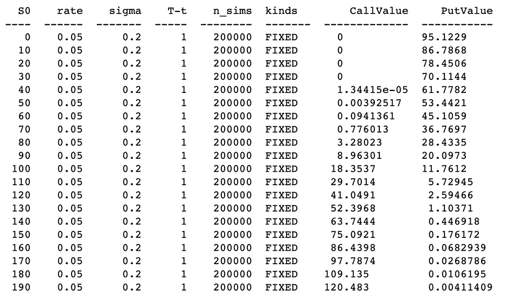
# Chart of Risk-free interest rate and option value
outdata = pd.DataFrame(ResultListLO, columns=HeaderLO)
outdata[['S0', 'CallValue','PutValue']].iplot(x='S0',
                                              y=['CallValue', 'PutValue'],
                                              mode='lines+markers',
                                              xTitle='S0',
                                              yTitle='Option Value',
                                              title='S0 and option value(FIXED)')
# Asian Option
ResultList = []
spath, ypath = asin_option(S0, r, sigma, horizon, mc_type='EM', n_sims=200000, vr_type='AV')
# Print the values
print(tabulate(ResultList, Header))

# Lookback Option (FLOATING)
ResultListLO = []
spath, ypath = lookback_option(S0, r, sigma, horizon, mc_type='EM', n_sims=200000, vr_type='AV', lo_type='FLOATING')

# Print the values
print(tabulate(ResultListLO, HeaderLO))

# Lookback Option (FIXED)
ResultListLO = []
spath, ypath = lookback_option(S0, r, sigma, horizon, mc_type='EM', n_sims=200000, vr_type='AV', lo_type='FIXED')

# Print the values
print(tabulate(ResultListLO, HeaderLO))
